
WHITEPAPER · VOLATILITY · October 2026
The Calm Before the Storm
Why historically low currency volatility does not reduce the risk in treasury portfolios – it only hides it.
Related: FX risk management for corporates The GLORIAnalytics platform
Key takeaways
- Implied three-month G10 volatility of 6.2% sits at the 12th percentile of its range since June 2022, and realised one-year EUR/USD volatility (5.5%) has been lower in only 4% of observations since 1999
- Geopolitical risk and currency volatility have decoupled: the Geopolitical Risk Index averages 188 points in 2026, almost twice its long-run mean, while currency volatility sits near its lows
- Every risk metric is at its core a volatility number: when volatility falls, reported risk falls with it without a single position changing – and hedge ratios, limits and budget ranges become procyclical
- In the sample portfolio of nine currencies, reported risk rises by a factor of 1.8 (from EUR 5.6 million to EUR 10.2 million) if volatility and correlation return to early-2023 levels
- Earlier calm periods (2007, 2014, 2019) each ended in a regime change within six to twelve months – five concrete steps a treasury can take now, without any forecast
Currency markets are quieter than they have been in years. In October 2026, implied three-month volatility across the G10 currencies averages 6.2% – the 12th percentile of the past four and a half years, and only just above July's low. Realised one-year volatility in EUR/USD stands at 5.5%, lower than in 96% of all observations since the euro was introduced. At the same time, the Geopolitical Risk Index is averaging 188 points for 2026, almost twice its long-run mean. That gap is the starting point of this paper.
For companies with foreign-currency exposure, the consequence is immediate. Every risk metric in use – value-at-risk, cash-flow-at-risk, peak risk – is at its core a volatility number. When volatility falls, reported risk falls with it, even though nothing has changed in the underlying positions. Our sample portfolio of nine currencies shows an annual risk of EUR 5.6 million today; with the volatility and correlation of early 2023 it would show EUR 10.2 million – on identical positions. A treasury that sets hedge ratios, limits or budget rates on the basis of today's numbers is calibrating its risk management to the quietest point in the cycle.
The paper proceeds in six steps: where volatility stands today; why calm must not be mistaken for safety; the mechanism that makes risk numbers procyclical; what happens to a realistic portfolio when the market changes regime; what earlier calm periods have taught us; and what a treasury can do now, while protection is still cheap. All figures come from our own calculations on daily market data; the methodology is documented in the appendix.
Where we stand: volatility in historical context
Volatility can be measured in two ways. Implied volatility is the price the options market charges today for future price swings – it is the market's expectation. Realised volatility is what actually happened: the standard deviation of daily moves over a past window. In October 2026 both tell the same story, with one nuance that matters.
Implied volatility: at the bottom of the range since 2022
Figure 1 shows the equal-weighted average of implied three-month and one-year volatility across eleven G10 currency pairs, from daily Fenics data. The picture is unambiguous. From a peak of 12.4% at the end of September 2022 – the energy crisis, the rate shock, the sterling crisis – implied volatility has come down in three steps. The tariff shock of April 2025 produced a brief spike to just over 10% that was unwound within weeks. Since the spring of 2026 the index has sat continuously below its interquartile band, reaching a low of 5.6% in mid-July. The current reading of 6.2% corresponds to the 12th percentile of the whole observation period; the median is 7.5%.
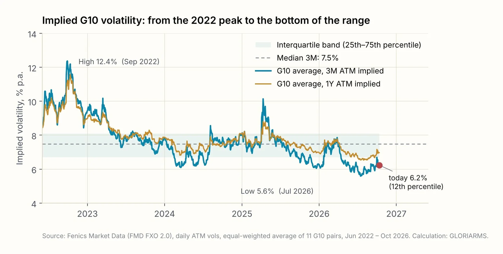
What is striking is that one-year volatility has followed the same path. At 7.0% it also sits at the 12th percentile. The market is not merely expecting calm for the next few weeks; it is pricing calm across the entire planning horizon of a typical hedging programme. That is the real reason why risk metrics in treasury systems that run on implied volatilities currently come out so low.
Not every pair, but the ones that matter
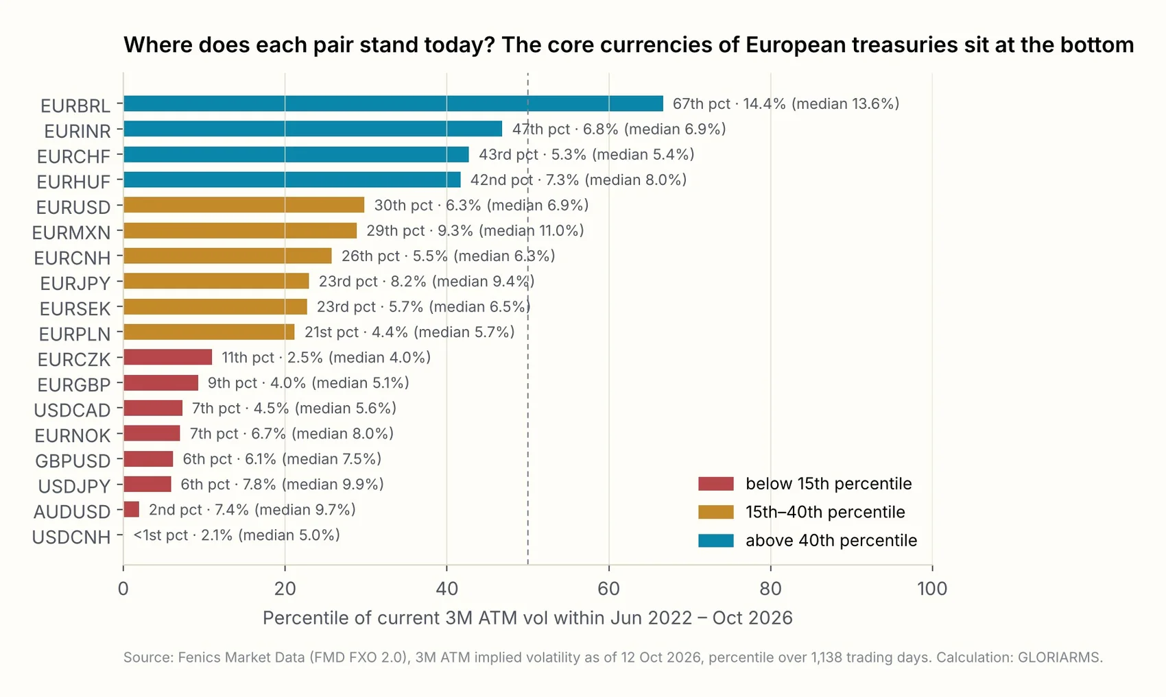
The picture is not uniform, and it would be dishonest to present it that way. Figure 2 ranks eighteen currency pairs by where their current three-month volatility sits within the range since June 2022. The red group – USD/CNH, AUD/USD, USD/JPY, GBP/USD, EUR/NOK, USD/CAD, EUR/GBP, EUR/CZK – is below the 15th percentile; USD/CNH, at 2.1%, is at the absolute low of the observation period. The middle group, which includes EUR/USD (30th percentile, 6.3%) and EUR/PLN, has moved off the summer lows but remains well below the median. At the top are a few emerging-market currencies such as BRL and INR, whose volatility is driven by local factors.
For a European treasury the decisive point is that the core currencies – USD, GBP, CHF, CNY, the Scandinavian currencies, CZK and PLN – all sit in the lower half, with GBP, NOK and CZK even in the bottom sixth. These are precisely the currencies that typically account for 80 to 90% of the exposure of a German or Italian industrial company.
Realised volatility: a 27-year perspective
Four and a half years of options data is a short yardstick, and it begins, awkwardly, in a stress period. To test the claim "historically low", we computed realised volatility from daily Federal Reserve spot rates going back to 1999 (Figure 3). The result is clearer than expected. Rolling three-month EUR/USD volatility stands at 5.0% – the 8th percentile since the euro's introduction, against a median of 8.6%. Over one year it is 5.5%, the 4th percentile. GBP/USD is at the 4th percentile with 5.2%; NOK and SEK against the dollar are similarly low. The only notable exception among the majors is USD/JPY, whose realised volatility of around 9.5% is close to its long-run median.
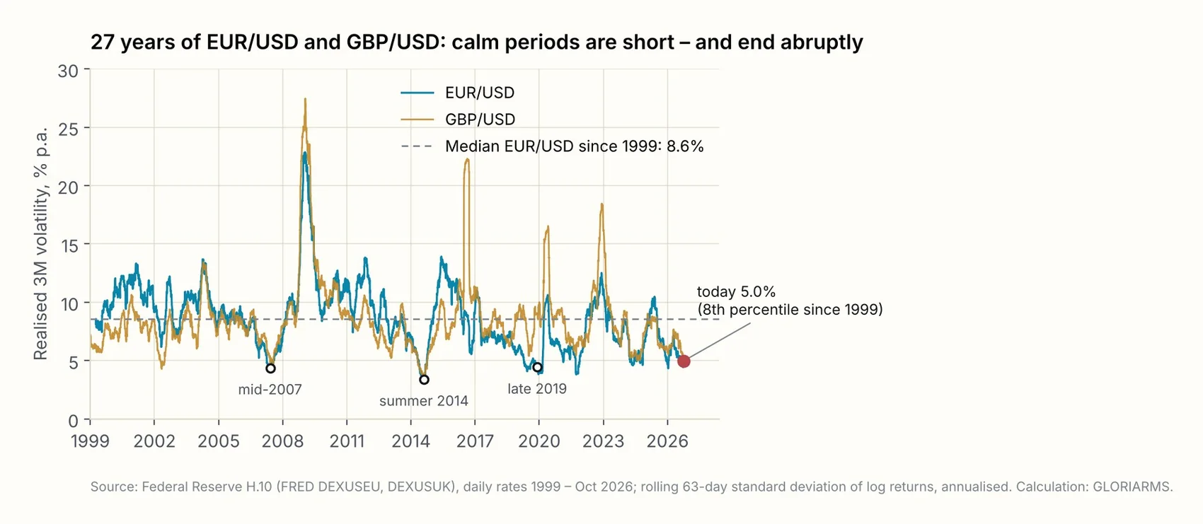
The chart shows something else. Since 1999 there have been only three episodes in which EUR/USD volatility fell below 6%: mid-2007, the summer of 2014 and late 2019. Each was followed within six to twelve months by a regime change – the financial crisis, the EUR/USD slide from 1.39 to 1.05 together with the abandonment of the Swiss franc floor, the pandemic. We return to these in section 05.
The nuance: implied sits above realised
Implied one-year EUR/USD volatility is 7.0%, close to its four-year median – realised is only 5.5%. The options market is therefore charging roughly 1.5 volatility points more than has recently materialised. This spread between implied and recently realised volatility is currently wide, and it is a first sign that the market itself does not entirely trust the calm. In practical terms: systems that compute risk from historical volatility currently report even lower numbers than those using implied volatilities. Both numbers are low; the historical one is more extreme.
The gap: geopolitics up, volatility down
Low volatility would be less remarkable if the world were quiet. It is not. Figure 4 sets the Geopolitical Risk Index of Caldara and Iacoviello – a newspaper-based measure of geopolitical tension that is well established in central-bank research – against the G10 volatility index. The GPR index averages 188 points in 2026; its long-run mean from 1985 to 2019 is normalised to 100. In the spring of 2026 the 30-day average exceeded 320, a level otherwise seen only in acute phases of war.
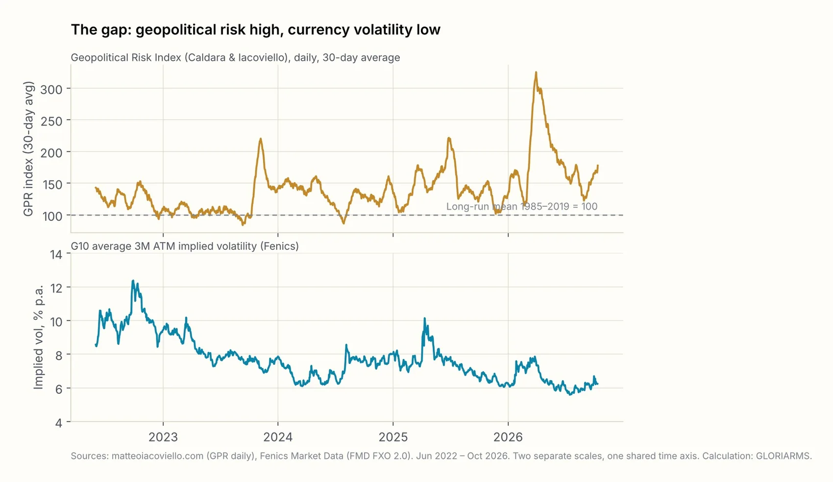
The two series have decoupled. In 2022 they still moved together; the rise in the GPR index in the autumn of 2023 found little echo in currency volatility, and the spike in the spring of 2026 coincided with volatility's low. There are three ways to read this. The first is habituation: markets have learned to look through geopolitical headlines as long as they have no direct consequences for interest rates and trade flows. The second is structural: interest-rate differentials between the major currency areas are small and stable, carry strategies dampen moves, and central banks act predictably. The third is a warning: the distance between what the market is pricing and what the world holds in risk has rarely been this large.
All three readings are defensible, and this paper does not presume to judge which is right. What matters for a treasury is that the second reading explains the stability of the calm but does not guarantee its duration. Rate differentials change; carry positions get unwound – and typically abruptly, as the yen demonstrated in August 2024, when USD/JPY fell twelve percent in three weeks and implied volatility doubled.
What the volatility curve and the skew are saying
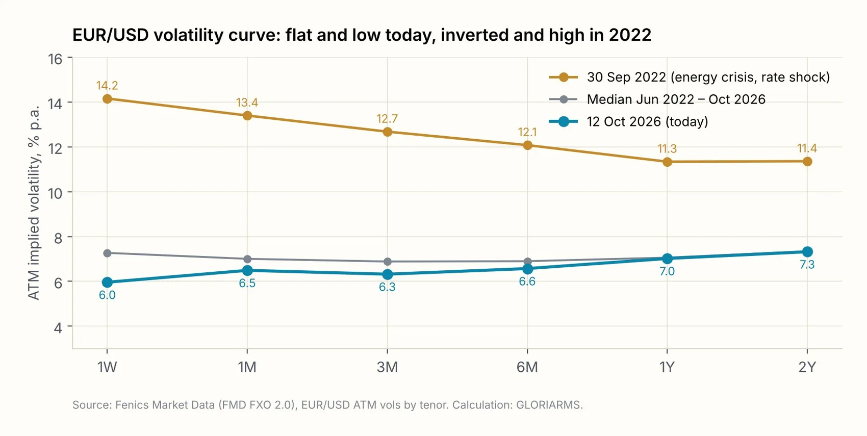
Two further market signals complete the picture. The term structure of EUR/USD volatility (Figure 5) is flat and gently upward-sloping today: 6.0% for one week, 7.3% for two years. In September 2022 it was inverted, with 14.2% at the front end – the market was then paying more for immediate protection than for long-dated cover. A flat, low curve is the signature of a phase in which nobody sees a specific trigger. That is exactly what makes it dangerous: the market is not pricing a date on which the calm ends, so any date will do.
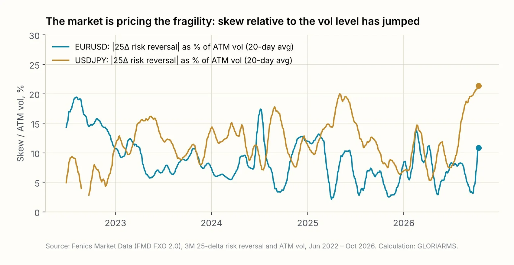
The skew – the price difference between options on appreciation and depreciation, measured by the 25-delta risk reversal – provides perhaps the most interesting signal. In absolute terms the risk reversals are unremarkable. Set against the level of ATM volatility, however (Figure 6), the market is charging as much for directional protection relative to the low ATM level as it rarely has before: in USD/JPY the skew amounts to 21% of ATM volatility, the 97th percentile since 2022; in EUR/USD the ratio has jumped within a few weeks from near zero to 11%, well above its median of 8%. The interpretation is simple. The options market is not expecting high volatility, but it considers the distribution of possible outcomes to be lopsided. The calm is priced in – and so is the fragility.
Why this matters to treasurers: risk numbers are volatility numbers
Every risk metric used in day-to-day treasury work reduces to the same formula: risk equals exposure times volatility times a confidence factor, supplemented at portfolio level by the correlations between currencies. Whether the number is called value-at-risk, cash-flow-at-risk, peak risk or earnings-at-risk, and whether it is computed parametrically, historically or by simulation, the prevailing market regime – and in particular the observed or priced-in volatility – shapes the result decisively.
That is not a weakness of the methodology; it is its definition. It becomes a problem only when the metric is used to make decisions that are meant to last longer than the volatility they were computed with. And that is exactly what happens in practice, in three places.
Hedge ratios become procyclical
Many hedging policies do not fix the hedge ratio outright but derive it from a risk limit: the open exposure may not exceed a given risk – say, five percent of planned EBIT. When volatility falls, more exposure fits under the limit at the same ratio, or the same positions permit a lower ratio. The system signals: you can hedge less. In the calm phase that is even arithmetically correct. But it means the hedge ratio is lowest precisely when protection would be cheapest – and has to be raised precisely when it is most expensive. This is the mechanism that forced many treasuries into the market in 2022 with volatility already at 12%.
Limits get used up without anyone deciding anything
A risk limit set in 2023 at EUR 10 million of peak risk is only half utilised in 2026 on the same positions. That invites the use of the free headroom – longer planning horizons, more currencies, less hedging. Each of these decisions is defensible on its own. Together they mean that economic risk rises while reported risk falls.
Budget rates and planning ranges become too narrow
Planning ranges for budget rates are frequently derived from implied or historical volatility. The loss threshold that EUR/USD will not exceed over twelve months with 95% probability – the value-at-risk logic – is around 9% at 5.5% volatility and around 18% at 11% volatility; a two-sided 95% band is correspondingly ±11% rather than ±22% wide. Anyone planning the 2027 budget on today's range has implicitly assumed that next year will be as quiet as the last. The historical evidence that extreme calm is followed by regime change argues against that assumption.
What happens when volatility comes back: a sample portfolio
To make the mechanism tangible, we defined a realistic exposure portfolio of a European industrial company, seen from the euro, and valued it with daily market data over the whole period since mid-2022. The portfolio holds nine currencies in mixed directions: export receivables in USD, GBP, JPY, CNY, MXN, BRL and INR, and procurement and production payables in CHF and PLN. The net twelve-month amounts are listed in the table. As the risk measure we use parametric value-at-risk at 95% confidence over one year, computed from the rolling covariance matrix of the past 252 trading days – a standard method that mirrors the logic of most treasury systems.
| Currency | Direction | Net exposure 12M (EUR m) | Vol today (1Y hist.) | Vol stress period 2023 |
|---|---|---|---|---|
| USD | Receivable | 40 | 5.5% | 9.4% |
| GBP | Receivable | 15 | 3.4% | 7.6% |
| CHF | Payable | −10 | 3.8% | 7.9% |
| JPY | Receivable | 8 | 6.6% | 12.7% |
| CNY | Receivable | 12 | 4.7% | 8.1% |
| PLN | Payable | −10 | 3.5% | 8.7% |
| MXN | Receivable | 6 | 6.0% | 9.9% |
| BRL | Receivable | 5 | 10.1% | 17.4% |
| INR | Receivable | 4 | 6.5% | 8.2% |
The same positions, half the risk
Figure 7 shows the path. Reported portfolio risk peaked in January 2023 at EUR 10.2 million, ran at a median of EUR 8.3 million over the past four years, and stands at EUR 5.6 million today – the 4th percentile of its own history. The positions have not changed. The entire decline is the result of lower volatility and, to a lesser extent, lower correlation.
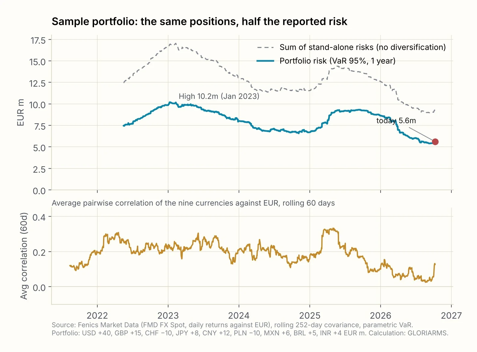
The lower panel deserves particular attention. The average correlation among the nine currencies – measured over rolling 60 days – fell to 0.04 in the third quarter of 2026, the lowest value of the whole period. During the 2022/23 stress phase it ran at 0.22; in the tariff crisis of May 2025 it briefly hit 0.33. Low correlation means a high diversification benefit: the portfolio looks today as if its currencies were hedging each other. That is the typical pattern of calm phases, in which each currency follows its own local themes. In stress it disappears, because a common factor – risk aversion, dollar demand, liquidity – then moves all currencies at once.
Four scenarios
Figure 8 decomposes the effect. We value the portfolio under four combinations of volatility and correlation: both as today; today's volatility with stress-period correlation; stress volatility with today's correlation; and both from the stress period. We also show a second portfolio with identical amounts but receivables only – that is, without the natural hedges provided by the CHF and PLN payables.
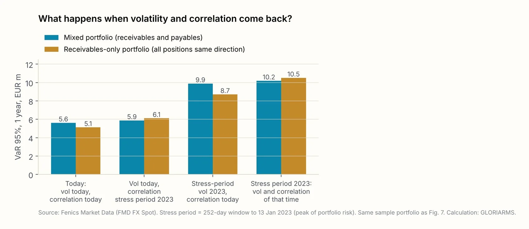
Two findings. First, the volatility effect dominates. If volatility returns to its early-2023 level, the risk of the mixed portfolio rises from EUR 5.6 million to EUR 9.9 million, a factor of 1.8 – and the 2023 level was no historical extreme; for EUR/USD it was close to the long-run median. Second, the correlation effect depends on the structure of the portfolio. For the mixed portfolio it is small, because the CHF and PLN payables act more strongly as natural hedges when correlation rises. For the receivables-only portfolio, the correlation jump to the May 2025 level alone lifts risk from EUR 5.1 million to EUR 6.8 million, by a third – before anything has changed in volatility. A portfolio in which all positions point the same way carries both risks, and they arrive together.
A note for systems that run on implied volatilities: with today's one-year market volatilities from Fenics, the risk of the mixed portfolio is EUR 7.3 million; with those of 30 September 2022 it would be EUR 12.4 million. The magnitude of the effect is the same; only the starting level is higher, because the options market – as described in section 01 – charges a premium over realised volatility.
Lessons from earlier calm periods
Figure 3 marked the three episodes since 1999 in which EUR/USD volatility stood roughly where it does today. It is worth a brief look at what followed in each case – not because history repeats itself, but because the mechanics of the transition were the same every time.
2007: In early summer, realised three-month EUR/USD volatility was around 5%, implied around 6%. The carry trade – funding in JPY and CHF, investing in high-yielding currencies – had dampened volatility for years. When the subprime crisis reached the first banks in August 2007, volatility doubled within three weeks; by January 2009 it had reached 23%. Companies that had lowered their hedge ratios in 2007 on the strength of the risk numbers of the time had to top up in the autumn of 2008 at the highest option premiums since the euro's introduction.
2014: In August 2014 EUR/USD volatility hit an all-time low of 3.4%; GBP/USD and USD/CHF were similarly low. The explanation was the same as today: central banks with clear forward guidance, low and stable rate differentials, no identifiable trigger. Over the following eight months EUR/USD fell from 1.39 to 1.05, the Swiss National Bank abandoned its floor in January 2015 – USD/CHF volatility went from 6% to over 30% in a single day – and implied EUR/USD volatility rose to 13%. The sample portfolio of section 04 would have more than doubled its reported risk over this period.
2019: At the end of 2019, realised EUR/USD volatility was 4.4%, the term structure was flat, and the US–China trade conflict was considered priced in. In March 2020 volatility jumped to over 14% within two weeks, correlations between all currencies against the dollar spiked, and for several weeks protection was available only at a multiple of its previous cost.
The pattern is the same in all three cases: a calm with sound structural reasons, a trigger that nobody had recognised as one beforehand, a transition measured in weeks rather than months – and hedging costs that were highest exactly when the need was greatest. None of these episodes could have been managed by forecasting. All of them could have been managed by preparation.
What a treasury can do now
The conclusion from the preceding sections is not that a crisis is imminent – we do not know that. It is that risk management should not be calibrated to the current volatility level, because that level has never lasted long in the past. Five concrete steps follow.
- Read risk numbers in regime comparison. Every peak-risk or CFaR figure should be shown alongside at least two reference values: the risk at the median volatility of the past five years, and the risk in the most recent stress period. Only the distance between these numbers tells you how much of today's calm is embedded in the reported risk. For our sample portfolio it is half.
- Anchor limits and ratios to stress volatility. A hedging policy that prescribes minimum ratios should set them so that the risk limit holds at stress volatility, not just at today's. In practice that means deliberately not lowering the ratio that today's low numbers would allow you to lower. In the calm phase that does not necessarily cost additional premium – but it does take discipline.
- Question the diversification assumption. Portfolios in which all positions point the same way currently benefit from a correlation near zero that disappears in stress. For such portfolios, risk should additionally be computed with the correlation of a stress period, and the difference tracked as a metric in its own right. Mixed portfolios with natural hedges are more robust here – an argument for looking at procurement and sales currencies together.
- Look at options while they are cheap. Low implied volatility means low option premiums. Option-based protection that was unaffordable in 2022 costs a fraction today. Hedging part of the exposure with options rather than forwards buys exactly what this paper describes: protection against a rise in volatility, without giving up all of the upside. Collars reduce the premium but cap part of that upside in return. The skew shows that the market is already charging more for directional protection – at the ATM level, however, it remains inexpensive.
- Match the monitoring rhythm to the height of the fall. Transitions out of calm periods have historically taken weeks. A quarterly risk report sees the transition only once it is over. Volatility, correlation and skew should be watched weekly in this phase, with defined thresholds that trigger a review of hedge ratios – for instance implied G10 volatility rising above its median, or average correlation jumping above 0.2.
None of these steps requires a forecast. All of them require the treasury to understand its risk numbers not as a measurement of risk, but as a measurement of risk under current market conditions – and to know how far those conditions are from normal.
How we make this visible for our clients
All analyses in this paper rest on the daily market data and the tools we use in GLORIAnalytics to value client portfolios. The percentile ranking of volatility by currency pair, the regime comparison of portfolio risk, and the correlation traffic light that sets historical against implied correlation are available there as running analyses. The peak-risk backtest shows, for a specific exposure, how reported risk would have evolved over recent years – and hence how much of today's figure is owed to the calm. The hedging laboratory allows hedge ratios and monitoring rhythms to be tested against market history before they are written into a policy.
If you would like to know where your own portfolio sits in this picture, we will gladly run the analysis of section 04 on your exposure.
Appendix: methodology and data
Option volatilities. Fenics Market Data, dataset FMD FXO 2.0, daily closing quotes (mid) of ATM volatility (delta-neutral) and 25-delta risk reversals for 22 tenors, 1 June 2022 to 12 October 2026, 1,138 trading days. The G10 index is the unweighted average of EUR/USD, USD/JPY, GBP/USD, USD/CHF, AUD/USD, USD/CAD, EUR/GBP, EUR/JPY, EUR/CHF, EUR/SEK and EUR/NOK. Percentiles refer to the distribution of daily values over the observation period.
Realised volatility. Daily noon rates of the Federal Reserve (H.10, series DEXUSEU, DEXUSUK, DEXJPUS, DEXSZUS and others), from 4 January 1999. Volatility as the standard deviation of log daily returns over 63 (three-month) or 252 (one-year) trading days, annualised by √252. Percentiles refer to all daily values since 1999.
Geopolitical Risk Index. Caldara, D. and M. Iacoviello (2022), "Measuring Geopolitical Risk", American Economic Review 112(4). Data downloaded from https://www.matteoiacoviello.com/gpr.htm on October 14, 2026 (daily and monthly series as of 13 October 2026; licence CC BY). The index counts articles on geopolitical tensions in ten major newspapers; the 1985–2019 mean is normalised to 100.
Sample portfolio. Daily returns of 56 currencies against EUR from Fenics spot rates (16:00 Berlin snapshot, mid), 24 May 2021 to 9 October 2026. Risk measure: parametric value-at-risk at 95% confidence (factor 1.645) over a one-year horizon, computed as the square root of the quadratic form of the position vector and the annualised covariance matrix of the trailing 252 trading days. The sum of stand-alone risks is the sum of the absolute stand-alone risks of all positions, ignoring diversification effects. The regime comparison in Figure 8 combines the volatility vectors and correlation matrices of two windows: the current one (to 9 October 2026) and the stress window (252 days to 13 January 2023, the peak of portfolio risk). The May 2025 correlation is the 60-day correlation matrix to 1 May 2025. The implied-based variant replaces historical volatilities with the one-year ATM volatilities from Fenics on the respective date. For the CNY exposure the onshore spot returns (EUR/CNY) are used; in the options analysis (Figures 2 and 8, implied variant) the more liquid offshore CNH volatility serves as the market proxy.
Limitations. The parametric method assumes normally distributed returns and therefore systematically understates tail risk – the actual height of the fall is, if anything, greater than shown. The observation period of the options data begins in a stress phase, which tends to bias percentiles upward relative to a longer history; the classification by realised volatility since 1999 is unaffected by this. The sample portfolio is an illustration, not a recommendation for any particular exposure structure.
GLORIARMS S.r.l. · Stefan Hamberger · This paper is for information purposes only and does not constitute investment or hedging advice. All calculations are based on the sources named; errors and omissions excepted. © 2026 GLORIARMS.
Frequently asked questions
How low is currency volatility in October 2026?
Implied three-month volatility across the G10 currencies averages 6.2% in October 2026 – the 12th percentile of its range since June 2022 (high: 12.4% in September 2022). Realised one-year EUR/USD volatility is 5.5% and has been lower in only 4% of observations since the euro was introduced. Data as of 12 October 2026, based on Fenics Market Data and Federal Reserve spot rates.
Does low volatility reduce the risk of a treasury portfolio?
No. It reduces the reported value of risk metrics such as value-at-risk, cash-flow-at-risk or peak risk, not the economic risk. In the sample portfolio of nine currencies, reported annual risk is EUR 5.6 million today; with the volatility and correlation of early 2023 it would be EUR 10.2 million on identical positions – an increase by a factor of 1.8.
Why do hedge ratios and limits become procyclical in calm markets?
Many hedging policies define the hedge ratio through a risk limit. When volatility falls, more exposure fits under the limit at the same ratio, so the ratio falls exactly when protection would be cheapest and has to be raised again when it is most expensive. A limit set at EUR 10 million of peak risk in 2023 is only half used on the same positions in 2026.
What do earlier calm periods such as 2007, 2014 and 2019 teach?
Realised EUR/USD volatility has been below 6% only three times since 1999: mid-2007, summer 2014 and end of 2019. Each was followed within six to twelve months by a regime change – the financial crisis, the end of the Swiss franc floor, the pandemic. The pattern is the same: a structurally justified calm, a trigger nobody had recognised as one, a transition within weeks, and hedging costs at their highest exactly when the need is greatest.
What can a treasury do now?
The paper names five steps that require no forecast: read risk numbers in a regime comparison (median volatility and the last stress phase), anchor limits and ratios to stress volatility, question the diversification assumption, look at options while they are cheap, and match the monitoring rhythm to the height of the fall – for example weekly instead of quarterly.
Which data and methods are the figures based on?
Option volatilities and risk reversals come from Fenics Market Data (FMD FXO 2.0, daily since 1 June 2022, 1,138 trading days), realised volatilities from Federal Reserve H.10 spot rates since 1999, and geopolitical risk from the Geopolitical Risk Index by Caldara and Iacoviello. The sample portfolio is valued with parametric value-at-risk (95%, one year) on the rolling 252-day covariance matrix. Methodology and limitations are in the appendix.
This whitepaper was drafted with AI-assisted research and writing tools and reviewed for accuracy and completeness by the authors below prior to publication.
Authors
